[1]:
import pdb,sys,os
import anndata
import scanpy as sc
sc.settings.verbosity = 0
import argparse
import copy
import numpy as np
import scipy

import timeit
import warnings
warnings.filterwarnings('ignore')

from matplotlib.pyplot import figure
import matplotlib.pyplot as plt
/mnt/data/jingtao2/anaconda3/envs/semi/lib/python3.9/site-packages/tqdm/auto.py:21: TqdmWarning: IProgress not found. Please update jupyter and ipywidgets. See https://ipywidgets.readthedocs.io/en/stable/user_install.html
  from .autonotebook import tqdm as notebook_tqdm
[2]:
import scSemiProfiler_dev as semidev
[3]:
from scSemiProfiler_dev.utils import *
Example
We provide an example dataset containing 12 samples from COVID-19 patients with 6 different severity levels. We will go through the process of using scSemiProfiler to semi-profile this example cohort. Then we will evaluate the semi-profiling performance by comparing the downstream anlaysis results using the semi-profiled cohort and the real-profiled cohort. We will show that even with only 2 representatives, we can accurately reproduce single-cell level downstream analysis results. Particularly, samples of different COVID-19 severity level can also be accurately inferred.
Step 1 Initial Setup
[4]:
name = 'runexample'
bulk = 'example_data/bulkdata.h5ad'
normed = 'yes'
geneselection = 'no'
batch = 2
[7]:
semidev.initsetup(name, bulk,normed,geneselection,batch)

'''
scSemiProfiler.initsetup.initsetup(name, bulk, normed = 'no',
geneselection = 'yes', batch = 4)

Parameters:
- name ('str'): Project name.
- bulk ('str'): Path to bulk data.
- normed ('str'): Whether the data has been library size normed or not.
- geneselection: ('str'): Whether to perform gene selection.
- batch ('str'): Representative selection batch size.

Returns:
- None
'''
Start initial setup
runexample exists. Please choose another name.
[7]:
"\nscSemiProfiler.initsetup.initsetup(name, bulk, normed = 'no', \ngeneselection = 'yes', batch = 4)\n\nParameters:\n- name ('str'): Project name. \n- bulk ('str'): Path to bulk data. \n- normed ('str'): Whether the data has been library size normed or not. \n- geneselection: ('str'): Whether to perform gene selection.\n- batch ('str'): Representative selection batch size.\n\nReturns:\n- None\n"
[11]:
_ = estimate_cost(12,2)

'''
estimate_cost():

Parameters:
- total_samples ('int'): The total number of samples in the cohort.
- n_representatives ('int'): The number of representative samples.

Returns:
- semicost ('float'): Estimated cost for semi-profiling.
- realcost ('float'): Estimated cost for conducting single-cell profiling for the entire cohort.
'''
Estimated semi-profiling cost: $11320.0
Estimated cost if conducting real single-cell profiling: $18000.0
Percentage saved: 37.1%
[11]:
"\nestimate_cost():\n\nParameters:\n- total_samples ('int'): The total number of samples in the cohort.\n- n_representatives ('int'): The number of representative samples.\n\nReturns:\n- semicost ('float'): Estimated cost for semi-profiling.\n- realcost ('float'): Estimated cost for conducting single-cell profiling for the entire cohort.\n"
Step 1.5 Acquiring Single-cell Data for Representatives
[12]:
semidev.get_eg_representatives(name)

'''
get_eg_representatives(name):

Parameters:
- name ('str'): Project name.

Returns:
None
'''
Obtained single-cell data for representatives.
[12]:
"\nget_eg_representatives(name):\n\nParameters:\n- name ('str'): Project name. \n\nReturns:\nNone\n"
Step 2 Single-cell Processing & Feature Augmentation
[5]:
semidev.scprocess(name=name,singlecell=name+'/representative_sc.h5ad',normed='yes',cellfilter='no',threshold=1e-3,geneset='yes',weight='yes',k=15)

'''
scSemiProfiler.scprocess.scprocess(name,singlecell,normed = 'no',
cellfilter = 'yes',threshold = 1e-3,geneset = 'human',weight = 0.5,
k = 15)

Parameters:
- name ('str'): Project name.
- singlecell ('str'): Path to representatives' single-cell data.
- normed ('str'): Whether the data has been library size normed or not.
- cellfilter: ('str'): Whether to perform cell selection.
- threshold ('float'): Threshold for background noise removal.
- geneset ('str'): Gene set file name.
- weight ('float'): The proportion of top features to increase importance weight.
- k ('int'): K for the K-NN graph built for cells.

Returns:
- None
'''
Processing representative single-cell data
Removing background noise
Computing geneset scores
GMT file c2.cp.v7.4.symbols.gmt loading ...
2922
Number of genes in c2.cp.v7.4.symbols.gmt 4240
KeyboardInterrupt
Step 3 Single-cell Inference
Pretrain 1: The model is trained to reconstruct the representatives’ single-cell data.
Pretrain 2: The model continues its reconstruction training in full batch mode, now incorporating an additional “representative bulk loss” term in the loss function. This term ensures that the reconstructed cells’ average expression is similar to pseudobulk.
Inference: The bulk data difference between the representative and target sample is integrated into the generator’s reconstruction process through a ‘target bulk loss’. This guides the generator to accurately infer the target sample’s cells.
Estimated Time for Samples with Approximately 7000 Cells: - Pretrain 1: 15 minutes per sample - Pretrain 2: 5 minutes per sample - Inference: 30 minutes per sample
[ ]:
1+1
[ ]:
representatives = name + '/status/init_representatives.txt'
cluster = name + '/status/init_cluster_labels.txt'

bulktype = 'pseudobulk'
semidev.scinfer(name, representatives,cluster,None,bulktype)

'''
scSemiProfiler.scinfer.scinfer(name, representatives, cluster,
targetid, bulktype = 'real', lambdad = 4.0, pretrain1batch = 128,
pretrain1lr = 1e-3, pretrain1vae = 100, pretrain1gan = 100,
lambdabulkr = 1, pretrain2lr = 1e-4, pretrain2vae = 50, pretrain2gan =
 50, inferepochs = 150, lambdabulkt = 8.0, inferlr = 2e-4, device = 'cuda:0')

Parameters:
- name ('str'): Project name.
- representatives ('str'): Path to the txt file recording this round of representative information.
- cluster ('str'): Path to the txt file recording this round of cluster label information.
- targetid: ('None'): Deprecated parameter for sanity check.
- bulktype ('str'): 'psedubulk' or 'real'. (Default: 'real')
- lambdad ('float'): Scaling factor for the discriminator loss.
- pretrain1batch ('int'): The mini-batch size during the first pretrain stage.
- pretrain1lr ('float'): The learning rate used in the first pretrain stage.
- pretrain1vae ('int'): The number of epochs for training the VAE during the first pretrain stage.
- pretrain1gan ('int'): The number of iterations for training GAN during the first pretrain stage.
- lambdabulkr ('float'): Scaling factor for represenatative bulk loss for pretrain 2.
- pretrain2lr ('float'): Pretrain 2 learning rate.
- pretrain2vae ('int'): The number of epochs for training the VAE during the second pretrain stage.
- pretrain2gan ('int'): The number of iterations for training the GAN during the second pretrain stage.
- inferepochs ('int'): The number of epochs used for each mini-stage during inference.
- lambdabulkt ('float'): Scaling factor for the initial target bulk loss.
- inferlr ('float'): Infer stage learning rate.
- device ('str'): Which device to use, e.g. 'cpu', 'cuda:0'.

Returns:
- None
'''
Start single-cell inference in cohort mode
pretrain 1: representative reconstruction
CUDA backend failed to initialize: Found CUDA version 11030, but JAX was built against version 11080, which is newer. The copy of CUDA that is installed must be at least as new as the version against which JAX was built. (Set TF_CPP_MIN_LOG_LEVEL=0 and rerun for more info.)
INFO Generating sequential column names
GPU available: True (cuda), used: True
TPU available: False, using: 0 TPU cores
IPU available: False, using: 0 IPUs
HPU available: False, using: 0 HPUs
You are using a CUDA device ('NVIDIA A16') that has Tensor Cores. To properly utilize them, you should set `torch.set_float32_matmul_precision('medium' | 'high')` which will trade-off precision for performance. For more details, read https://pytorch.org/docs/stable/generated/torch.set_float32_matmul_precision.html#torch.set_float32_matmul_precision
LOCAL_RANK: 0 - CUDA_VISIBLE_DEVICES: [0,1,2,3,4,5,6,7]
Epoch 5/100: 4%| | 4/100 [00:09<04:11, 2.62s/it, v_num=1, train_loss_step=912, t
Performance evaluation
After the inference is finished for the cohort, we first perform some basic visualization to see if the model training was successful.
[ ]:
repres = []
f=open(name + '/status/init_representatives.txt','r')
lines = f.readlines()
f.close()
for l in lines:
    repres.append(int(l.strip()))

cl = []
f=open(name + '/status/init_cluster_labels.txt','r')
lines = f.readlines()
f.close()
for l in lines:
    cl.append(int(l.strip()))
Reconstruction
Firstly, successful pretrain should generate near perfect reconstruction. We compare the representative’s reconstructed cells with the original ones.
[5]:
visualize_recon(name, 6)

'''
visualize_recon(name, representative = 6)

Parameters:
- name ('str'): Project name.
- representative ('int'): Specifying the representative to visualize.

Returns:
None
'''
CUDA backend failed to initialize: Found CUDA version 11030, but JAX was built against version 11080, which is newer. The copy of CUDA that is installed must be at least as new as the version against which JAX was built. (Set TF_CPP_MIN_LOG_LEVEL=0 and rerun for more info.)
INFO Generating sequential column names

The overlap indicates the reconstructed cells and representative cells are similar.
Target sample inference
Then, for any target sample, successful inference should generate target cells closer to the target ground truth than to the representative cells.
[6]:
visualize_inferred(name, 0, repres, cl)

'''
visualize_inferred(name, target, representatives, cluster_labels)

Parameters:
- name ('str'): Project name.
- target ('int'): Specifying the target to visualize.
- representatives ('list'): The list of representatives.
- cluster_labels ('list'): The list of cluster labeles.

Returns:
None
'''

The overlap between the target inferred cells and target ground truth indicates good inference performance.
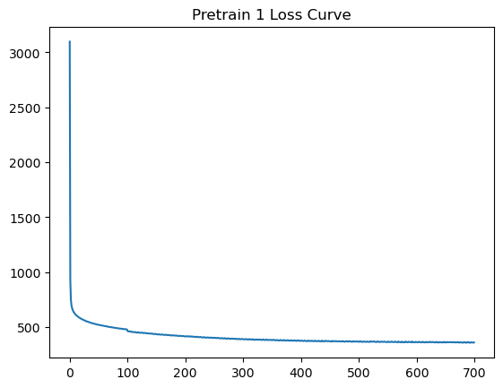
Check training loss curve
visualizing the loss curve during training:
[7]:
# PRETRAIN 1
# select a representative and check pretrain 1 loss curve
loss_curve(name, reprepid='BGCV09_CV0279',tgtpid=None,stage=1) # or loss_curve(name, sids, reprepid=6,tgtpid=None,stage=1)

'''
loss_curve(name, reprepid=None, tgtpid=None, stage=1)

Parameters:
- name ('str'): Project name.
- reprepid ('int'): Specifying the representative.
- tgtpid ('int'): The target sample. (not necessary for pretrain stages)
- stage ('int'): Specifying the training stage. (1: pretrain 1; 2: pretrain 2; 3: inference)

Returns:
None
'''
[8]:
# PRETRAIN 2
loss_curve(name, reprepid='BGCV09_CV0279',tgtpid=None,stage=2)

[9]:
# INFERENCE
# target bulk loss during 5 ministages for inference
loss_curve(name, reprepid=6,tgtpid=1,stage=3)

Comprehensive evaluation using more downstream tasks
We can assemble the representatives’ single-cell data and all inferred single-cell data into a semi-profiled cohort and use it to do all kinds of single-cell analysis. We compare the analysis results generated using the real-profiled cohort and semi-profiled cohort to evaluate the performance of semi-profiling.
Assemble semi-profiled cohort
(training an MLP to annotate the cell types takes around 5 minutes)
[13]:
representatives = repres
cluster_labels = cl
semisdata = assemble_cohort(name,
                representatives,
                cluster_labels,
                celltype_key = 'celltypes',
                sample_info_keys = ['states_collection_sum'])

'''
assemble_cohort(name,
                representatives,
                cluster_labels,
                celltype_key = 'celltypes',
                sample_info_keys = ['states_collection_sum'])

Parameters:
- name ('str'): Project name.
- representatives ('Union[list, str]'): A list of representatives or path to a txt file specifying the representatives.
- cluster_labels ('Union[list, str]'): A list of cluster labels or path to a txt file specifying the cluster labels.
- celltype_key ('str'): The key in anndata.AnnData.obs specifying the cell types.
- sample_info_keys ('list'): The other keys for sample informations that needs to be preserved in the semi-profiled dataset.

Returns:
semidata ('anndata.AnnData'): The semi-profiled cohort with cell type annotated.
'''
Start assembling semi-profiled cohort.
Training cell type annotator.
Finished. Cost 189.30423514000722 seconds.
Generating semi-profiled cohort data.
Finished assembling semi-profiled cohort. Output as semidata.h5ad
Read the real-profiled single-cell data to compare to
[14]:
gtdata = anndata.read_h5ad('example_data/scdata.h5ad')
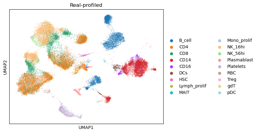
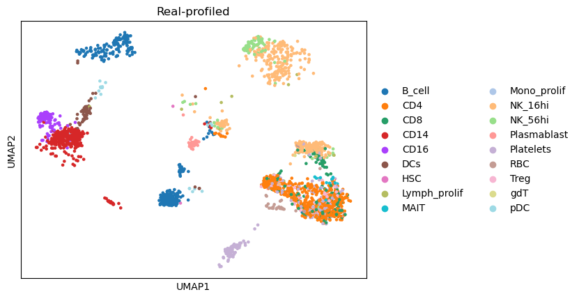
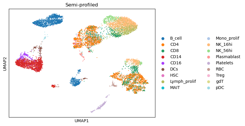
Compare the UMAP visualization
(The dimensionality reduction and neighbor graph calculation could be slow, taking around 5 minutes)
[18]:
st= timeit.default_timer()
combined_data,gtdata,semidata = compare_umaps(
            semidata = semisdata,
            name = name,
            representatives = name + '/status/init_representatives.txt',
            cluster_labels = name + '/status/init_cluster_labels.txt',
            celltype_key = 'celltypes'
            )

'''
compare_umaps(
                semidata,
                name = 'testexample',
                representatives = 'testexample/status/init_representatives.txt',
                cluster_labels = 'testexample/status/init_cluster_labels.txt',
                celltype_key = 'celltypes'
             )

Parameters:
- semidata ('anndata.AnnData'): The semi-profiled cohort.
- name ('str'): Project name.
- representatives ('Union[list, str]'): A list of representatives or path to a txt file specifying the representatives.
- cluster_labels ('Union[list, str]'): A list of cluster labels or path to a txt file specifying the cluster labels.
- celltype_key ('str'): The key in anndata.AnnData.obs specifying the cell types.

Returns:
- combdata ('anndata.AnnData'): The combined dataset with UMAP stored.
- gtdata ('anndata.AnnData'): The ground truth real-profiled dataset with UMAP stored.
- semidata ('anndata.AnnData'): The semi-profiled datset with UMAP stored.
'''


Compare cell type composition
[24]:
totaltypes = np.array(semisdata.obs['celltypes'].cat.categories)
gtprop = celltype_proportion(gtdata,totaltypes)
semiprop = celltype_proportion(semisdata,totaltypes)

'''
celltype_proportion(adata,totaltypes):

Parameters:
- adata ('anndata.AnnData'): An annotated dataset.
- totaltypes ('numpy.ndarray'): The names of all cell types.

Returns:
- prop ('numpy.ndarray'): The proportion of all cell types.
'''

print('Pearson Correlation between the two versions of cell type proportions:')
print(scipy.stats.pearsonr(gtprop,semiprop))
Pearson Correlation between the two versions of cell type proportions:
PearsonRResult(statistic=0.9842350182723907, pvalue=1.8260656886315043e-13)
[27]:
groupby = 'states_collection_sum'
composition_by_group(
    adata = gtdata,
    groupby = groupby,
    title = 'Ground truth'
    )

'''
composition_by_group(
    adata,
    colormap = None,
    groupby = None,
    save = False,
    title = 'Cell type composition'
    )

Parameters:
- adata ('anndata.AnnData'): An cell type annotated dataset.
- colormap ('numpy.ndarray'): The colormap used in visualization.
- groupby ('str'): The key specifying the grouping of cells. The plot will create a bar for each group.
- save ('Union[Bool,str]'): A path specifying where to save the plot or Boolean value.
- title ('str'): The title of the generated plot.

Returns:
None
'''
[28]:
groupby = 'states_collection_sum'
composition_by_group(
    adata = semisdata,
    groupby = groupby,
    title = 'Semi-profiled'
    )

Compare gene set activation pattern
We use the interferon pathway used in the COVID-19 study as an example.
[29]:
#https://www.gsea-msigdb.org/gsea/msigdb/cards/GO_RESPONSE_TO_TYPE_I_INTERFERON
IFN_genes = ["ABCE1", "ADAR", "BST2", "CACTIN", "CDC37", "CNOT7", "DCST1", "EGR1", "FADD", "GBP2",  "HLA-A",        "HLA-B",        "HLA-C",        "HLA-E",        "HLA-F",        "HLA-G",        "HLA-H",        "HSP90AB1",     "IFI27",        "IFI35",        "IFI6",         "IFIT1",        "IFIT2",        "IFIT3",        "IFITM1",       "IFITM2",       "IFITM3",       "IFNA1",        "IFNA10",       "IFNA13",       "IFNA14",       "IFNA16",       "IFNA17",       "IFNA2",        "IFNA21",       "IFNA4",        "IFNA5",        "IFNA6",        "IFNA7",        "IFNA8",        "IFNAR1",       "IFNAR2",       "IFNB1",        "IKBKE",        "IP6K2",        "IRAK1",        "IRF1",         "IRF2",         "IRF3",         "IRF4",         "IRF5",         "IRF6",         "IRF7",         "IRF8",         "IRF9",         "ISG15",        "ISG20",        "JAK1",         "LSM14A",       "MAVS",         "METTL3",       "MIR21",        "MMP12",        "MUL1",         "MX1",  "MX2",  "MYD88",        "NLRC5",        "OAS1",         "OAS2",         "OAS3",         "OASL",         "PSMB8",        "PTPN1",        "PTPN11",       "PTPN2",        "PTPN6",        "RNASEL",       "RSAD2",        "SAMHD1",       "SETD2",        "SHFL",         "SHMT2",        "SP100",        "STAT1",        "STAT2",        "TBK1",         "TREX1",        "TRIM56",       "TRIM6",        "TTLL12",       "TYK2",         "UBE2K",        "USP18",        "WNT5A", "XAF1", "YTHDF2", "YTHDF3", "ZBP1"]
[34]:
gtmtx = geneset_pattern(gtdata,IFN_genes,'states_collection_sum','celltypes')

'''
geneset_pattern(
adata,
genes,
condition_key,
celltype_key,
baseline=None,
)

Parameters:
- adata ('anndata.AnnData'): An cell type annotated dataset.
- genes ('list'): The list of gene in the gene set for computing the score.
- condition_key ('str'): The key in '.obs' specifying the condition.
- celltype_key ('str'): The key in '.obs' specifying the cell type.
- baseline ('str'): The base line condition to compare.

Returns:
None
'''
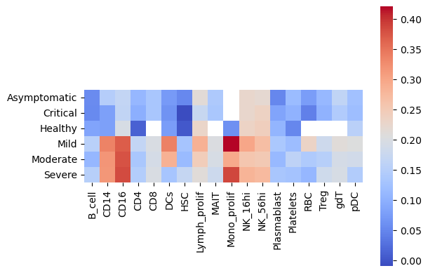
[36]:
if semisdata.X.max() > 20:
    sc.pp.log1p(semisdata)
[37]:
semismtx = geneset_pattern(semisdata,IFN_genes,'states_collection_sum','celltypes')
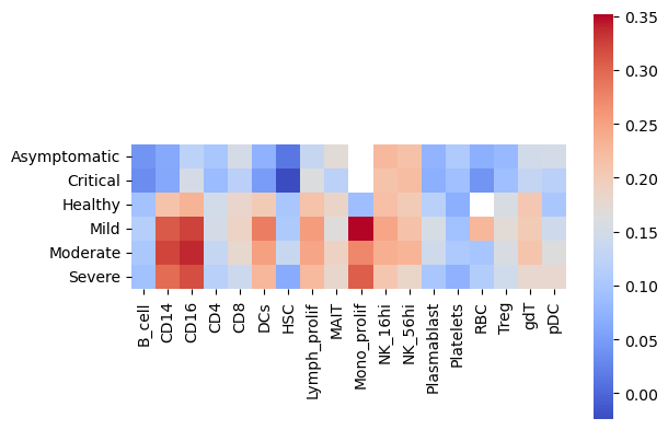
[53]:
print('Correlation between the two heatmaps:')
scipy.stats.pearsonr(np.nan_to_num(gtmtx.flatten(),0),np.nan_to_num(semismtx.flatten(),0))
Correlation between the two heatmaps:
[53]:
PearsonRResult(statistic=0.824605073506332, pvalue=5.559004210779983e-28)
Based on only 2 representatives, the semi-profiled data reproduces the pattern for all COVID-19 severity levels accurately.
Compare top cell type signature genes
[38]:
celltype_signature_comparison(gtdata=gtdata,semisdata=semisdata,celltype_key='celltypes')

'''
celltype_signature_comparison(gtdata, semisdata, celltype_key)

Parameters:
- gtdata ('anndata.AnnData'): The real-profiled ground truth dataset.
- semidata ('anndata.AnnData'): The semi-profiled dataset.
- celltype_key ('str'): The key in '.obs' specifying the cell type.

Returns:
None
'''
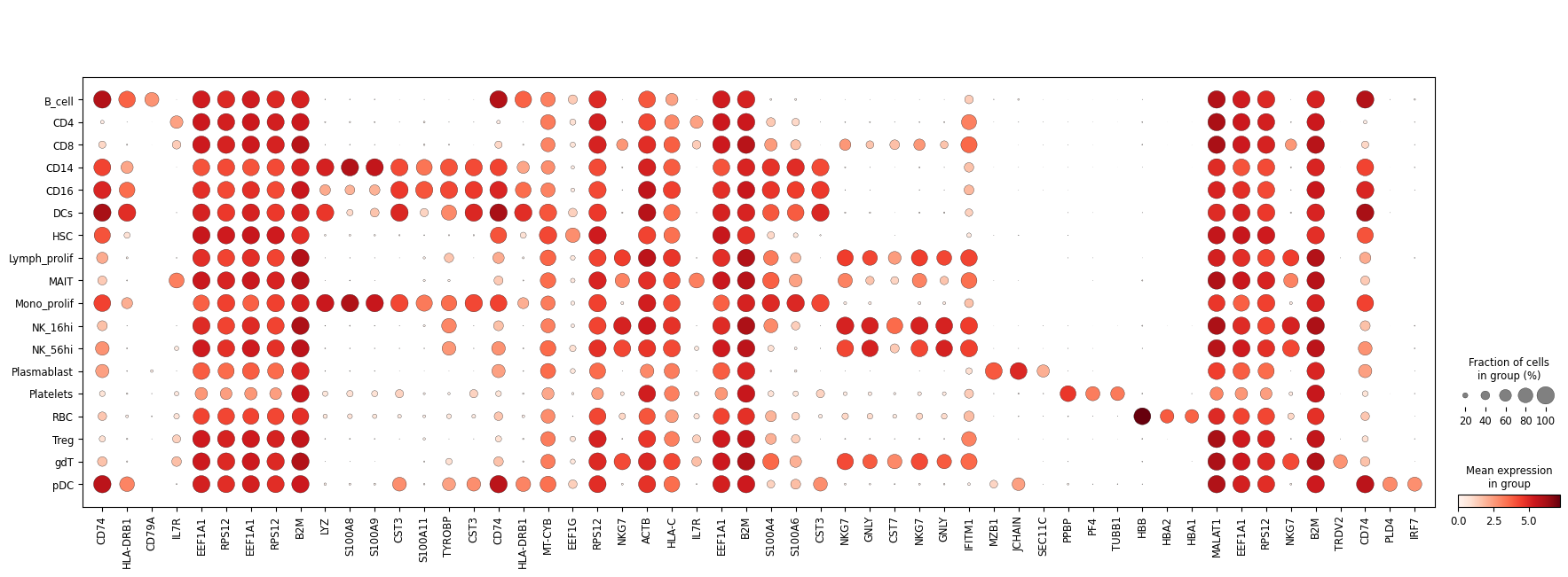

Expression fraction (size) similarity between real and semi-profiled:
PearsonRResult(statistic=0.9825868563126193, pvalue=0.0)
Expression intensity (color) similarity between real and semi-profiled
PearsonRResult(statistic=0.9886825546484544, pvalue=0.0)
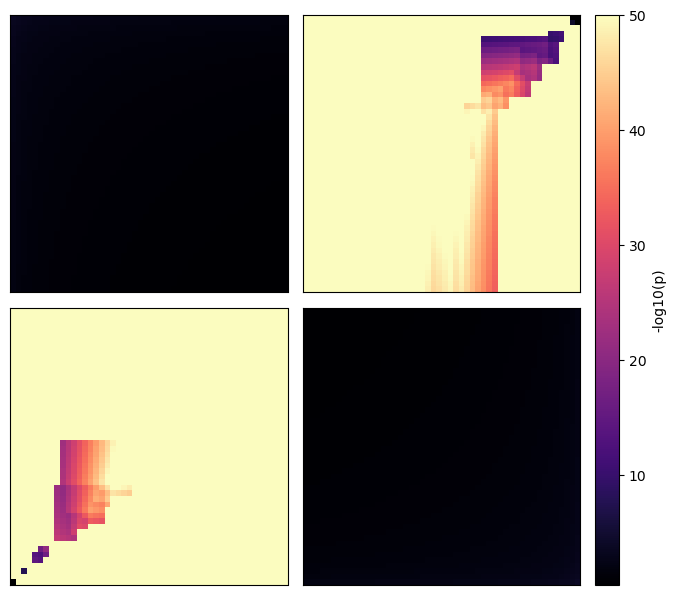
Use RRHO plot to compare markers
[40]:
# choose any cell type
print(totaltypes)
selected_celltype = 'CD4'
['B_cell' 'CD4' 'CD8' 'CD14' 'CD16' 'DCs' 'HSC' 'Lymph_prolif' 'MAIT'
 'Mono_prolif' 'NK_16hi' 'NK_56hi' 'Plasmablast' 'Platelets' 'RBC' 'Treg'
 'gdT' 'pDC']
[42]:
rrho(gtdata=gtdata,semisdata=semisdata,celltype_key='celltypes',celltype=selected_celltype)

'''
rrho(gtdata, semisdata, celltype_key, celltype)

Parameters:
- gtdata ('anndata.AnnData'): The real-profiled ground truth dataset.
- semidata ('anndata.AnnData'): The semi-profiled dataset.
- celltype_key ('str'): The key in '.obs' specifying the cell type.
- celltype ('str'): The cell type to analyze.

Returns:
None
'''
Plotting RRHO for comparing CD4 markers.
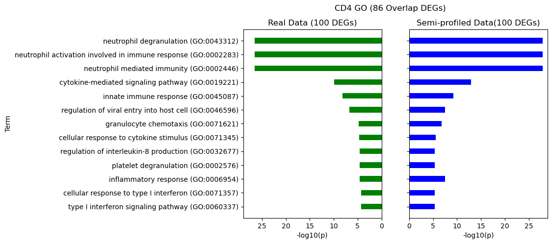
Compare GO enrichment analysis similarity
[46]:
selected_celltype = 'CD4'
enrichment_comparison(name, gtdata, semisdata, celltype_key = 'celltypes', selectedtype = selected_celltype)

'''
enrichment_comparison(name, gtdata, semisdata, celltype_key, selectedtype)

Parameters:
- name ('str'): Project name.
- gtdata ('anndata.AnnData'): The real-profiled dataset.
- semisdata ('anndata,AnnData'): The semi-profiled dataset.
- celltype_key ('str'): The key in '.obs' specifying the cell type.
- selectedtype ('str'): The cell type to analyze.

Returns:
None
'''
p-value of hypergeometric test for overlapping DEGs: 2.503329243550031e-165
Significance correlation: PearsonRResult(statistic=0.9965959843736519, pvalue=2.81960927017642e-13)
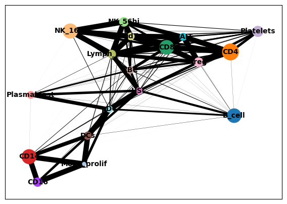
Compare partition-based graph abstraction (PAGA) graph similarity
[48]:
# GROUND TRUTH
threshold = 0
sc.tl.pca(gtdata,n_comps=100)
sc.pp.neighbors(gtdata,use_rep='X_pca',n_neighbors=50)
sc.tl.paga(gtdata, groups = 'celltypes')
sc.pl.paga(gtdata, plot=True,threshold=threshold)
[49]:
# SEMI-PROFILED
threshold = 0
sc.tl.pca(semisdata,n_comps=100)
sc.pp.neighbors(semisdata,use_rep='X_pca',n_neighbors=50)
sc.tl.paga(semisdata, groups = 'celltypes')
sc.pl.paga(semisdata, plot=True,threshold=threshold)

[50]:
gtpaga = np.array(gtdata.uns['paga']['connectivities'].todense())
semipaga = np.array(semisdata.uns['paga']['connectivities'].todense())
gtpaga = gtpaga.reshape((-1))
semipaga= semipaga.reshape((-1))
print('Correlation between the two adjacency matrices:')
scipy.stats.pearsonr(gtpaga,semipaga)
Correlation between the two adjacency matrices:
[50]:
PearsonRResult(statistic=0.847876215624918, pvalue=9.702626948663493e-91)
Using CellChat to perform cell-cell interaction analysis
conda create -n r_analysis r-essentials r-base
Activate it:
conda activate r_analysis
Start an interactive R session:
R
Install necessary packages:
1
install.packages('devtools')
2
if (!require("BiocManager", quietly = TRUE))
    install.packages("BiocManager")

BiocManager::install("Biobase")
3
if (!require("BiocManager", quietly = TRUE))
    install.packages("BiocManager")

BiocManager::install("ComplexHeatmap")
4
if (!require("BiocManager", quietly = TRUE))
    install.packages("BiocManager")

BiocManager::install("BiocNeighbors")
5
devtools::install_github("sqjin/CellChat")
Then install this R environment as a Jupyter Notebook kernel:
install.packages('IRkernel')
IRkernel::installspec(user = TRUE)
This finishes configuring the environment needed. You should be able to select the ‘R’ kernel in Jupyter Notebook. We will export some single-cell data for cell-cell interaction analysis.
Export single-cell data for analysis
We export real and semi-profiled cells from moderate COVID-19 patients.
[82]:
condition_real = gtdata[gtdata.obs['states_collection_sum'] == 'Moderate']
condition_semi = semisdata[semidata.obs['states_collection_sum'] == 'Moderate']
condition_real.write(name + '/moderate_real.h5ad')
condition_semi.write(name + '/moderate_semi.h5ad')
Then please open our notebook “cellchat_eg.ipynb” to proceed with the analysis.
End of comprehensive semi-profiling performance evaluation
Based on only two representative samples, the semi-profiled 12-sample cohort has very similar downstream analysis results as the real-profiled cohort, which contains heterogeneous samples from 6 different COVID-19 severity levels.
Optional: New Representative Selection and Run the Next Round
You have the option to employ active learning for the selection of additional representatives. This approach can result in some target samples having more similar representatives, thereby enhancing the accuracy of the inference process.
Round 2 semi-profiling
select a new batch of representatives using active learning:
[8]:
representatives = 'testrun/status/init_representatives.txt'
cluster = 'testrun/status/init_cluster_labels.txt'
targetid = None
bulktype = 'pseudobulk'
[13]:
activeselect.activeselection(name, representatives,cluster,batch=2,lambdasc=1,lambdapb=1)

'''
scSemiProfiler.activeselection.activeselection(name, representatives,
 cluster, batch, lambdasc, lambdapb)

Parameters:
- name ('str'): Project name.
- representatives ('str'): A `.txt` file specifying the representatives.
- cluster ('str'): A `.txt` file specifying the cluster labels.
- batch: ('int'): Representative selection batch size.
- lambdasc ('float'): Scaling factor for the single-cell transformation difficulty from the representative to the target.
- lambdapb ('float'): Scaling factor for the pseudobulk data.difference.

Returns:
- None
'''
Running active learning to select new representatives
selection finished
obtain single-cell data for new representatives:
[14]:
get_eg_representatives.get_eg_representatives(name)
[15]:
scprocess.scprocess(name=name,singlecell=name+'/representative_sc.h5ad',normed='yes',cellfilter='no',threshold=1e-3,geneset='yes',weight='yes',k=15)
Processing representative single-cell data
Removing background noise
Computing geneset scores
GMT file c2.cp.v7.4.symbols.gmt loading ...
2922
Number of genes in c2.cp.v7.4.symbols.gmt 4240
GMT file c2.cp.v7.4.symbols.gmt loading ...
2922
Number of genes in c2.cp.v7.4.symbols.gmt 4240
GMT file c2.cp.v7.4.symbols.gmt loading ...
2922
Number of genes in c2.cp.v7.4.symbols.gmt 4240
GMT file c2.cp.v7.4.symbols.gmt loading ...
2922
Number of genes in c2.cp.v7.4.symbols.gmt 4240
Augmenting and saving single-cell data.
Finished processing representative single-cell data
run single-cell inference again with more representatives:
[57]:
representatives = name + '/status/eer_representatives_2.txt'
cluster = name + '/status/eer_cluster_labels_2.txt'
bulktype = 'pseudobulk'

scinfer(name, representatives, cluster, None, bulktype)
Start single-cell inference in cohort mode
pretrain 1: representative reconstruction
load existing pretrain 1 reconstruction model for BGCV09_CV0279
INFO     Generating sequential column names
load existing pretrain 1 reconstruction model for MH9143426
INFO     Generating sequential column names
load existing pretrain 1 reconstruction model for BGCV07_CV0137
INFO     Generating sequential column names
load existing pretrain 1 reconstruction model for MH8919226
INFO     Generating sequential column names
pretrain2: reconstruction with representative bulk loss
load existing model
load existing pretrain 2 model for BGCV09_CV0279
INFO     Generating sequential column names
load existing model
load existing pretrain 2 model for MH9143426
INFO     Generating sequential column names
load existing model
load existing pretrain 2 model for BGCV07_CV0137
INFO     Generating sequential column names
load existing model
load existing pretrain 2 model for MH8919226
INFO     Generating sequential column names
inference
Inference for AP8 has been finished previously. Skip.
Inference for BGCV02_CV0068 has been finished previously. Skip.
Inference for BGCV03_CV0084 has been finished previously. Skip.
Inference for BGCV03_CV0176 has been finished previously. Skip.
Inference for BGCV04_CV0164 has been finished previously. Skip.
Inference for MH8919227 has been finished previously. Skip.
Inference for MH9143322 has been finished previously. Skip.
Inference for newcastle20 has been finished previously. Skip.
Finished single-cell inference
stop criteria
In real world application, you do not have the ground truth data for evaluating semi-profiling performance. But you can decide if you want to stop or continue semi-profiling with more representatives based on your budget, or evaluating the semi-profiling performance by comparing the representatives and their inferred data in the previous round.
[89]:
## GET REAL AND INFERRED NEW REPRESENTATIVES:

real_rep, inferred_rep = assemble_representatives(name,celltype_key='celltypes',sample_info_keys = ['states_collection_sum'],rnd=2,batch=2)

'''
assemble_representatives(name,celltype_key='celltypes',sample_info_keys = ['states_collection_sum'],rnd=2,batch=2)

Parameters:
- name ('str'): Project name.
- celltype_key ('str'): The key specifying the cell type.
- sample_info_key ('list'): The other sample information keys to be preserved in the generated dataset.
- rnd ('int'): The round of semi-profiling.
- batch ('int'): The batch size of representative selection.

Returns:
- realrepdata ('anndata.AnnData'): The real-profiled representative data.
- infrepdata ('anndata.AnnData'): The semi-profiled representative data.
'''
Training cell type annotator.
Finished. Cost 201.21513223499642 seconds.
then you can compare them using any of the anlaysis tasks shown previously, e.g UMAP, deconvolution.
[92]:
_ = compare_adata_umaps(
    inferred_rep,
    real_rep,
    name = name,
    celltype_key = 'celltypes'
    )

'''
compare_adata_umaps(
semidata,
gtdata,
name = 'testexample',
celltype_key = 'celltypes')

Parameters:
- semidata ('anndata.AnnData'): Semi-profiled dataset.
- gtdata ('anndata.AnnData'): Real-profiled dataset.
- name ('str'): Project name.
- celltype_key ('str'): The key specifying the cell type.

Returns:
- combdata ('anndata.AnnData'): Combined data with UMAP stored.
- gtdata ('anndata.AnnData'): Real-profiled data with UMAP stored.
- semidata ('anndata.AnnData'): Semi-profiled data with UMAP stored.
'''

[91]:
totaltypes = np.array(inferred_rep.obs['celltypes'].cat.categories)
real_prop = celltype_proportion(real_rep,totaltypes)
inferred_prop = celltype_proportion(inferred_rep,totaltypes)
print('Pearson Correlation between the two versions of cell type proportions:')
print(scipy.stats.pearsonr(real_prop,inferred_prop))
Pearson Correlation between the two versions of cell type proportions:
PearsonRResult(statistic=0.9188102942534281, pvalue=7.341435677365842e-08)
A Pearson Correlation of 0.918 is generally considered as good deconvolution performance. So if your are mainly focusing on cell type-level analysis then you can stop here. If you are not satisfied with it or not satisfied with more in-depth analysis results, you can select more representatives and go to the next round.
new representative selection using active learning
[86]:
activeselect.activeselection(name, representatives,cluster,batch=2,lambdasc=1,lambdapb=1)
Running active learning to select new representatives
selection finished
Round 3 semi-profiling
[69]:
get_eg_representatives.get_eg_representatives(name)
scprocess.scprocess(name=name,singlecell=name+'/representative_sc.h5ad',normed='yes',cellfilter='no',threshold=1e-3,geneset='yes',weight='yes',k=15)
[70]:
representatives = name + '/status/eer_representatives_3.txt'
cluster = name + '/status/eer_cluster_labels_3.txt'
scinfer(name, representatives,cluster,None,bulktype,device = 'cuda:0')
Start single-cell inference in cohort mode
pretrain 1: representative reconstruction
load existing pretrain 1 reconstruction model for BGCV09_CV0279
INFO     Generating sequential column names
load existing pretrain 1 reconstruction model for MH9143426
INFO     Generating sequential column names
load existing pretrain 1 reconstruction model for BGCV07_CV0137
INFO     Generating sequential column names
load existing pretrain 1 reconstruction model for MH8919226
INFO     Generating sequential column names
load existing pretrain 1 reconstruction model for BGCV03_CV0084
INFO     Generating sequential column names
load existing pretrain 1 reconstruction model for AP8
INFO     Generating sequential column names
pretrain2: reconstruction with representative bulk loss
load existing model
load existing pretrain 2 model for BGCV09_CV0279
INFO     Generating sequential column names
load existing model
load existing pretrain 2 model for MH9143426
INFO     Generating sequential column names
load existing model
load existing pretrain 2 model for BGCV07_CV0137
INFO     Generating sequential column names
load existing model
load existing pretrain 2 model for MH8919226
INFO     Generating sequential column names
load existing model
load existing pretrain 2 model for BGCV03_CV0084
INFO     Generating sequential column names
load existing model
load existing pretrain 2 model for AP8
INFO     Generating sequential column names
inference
Inference for BGCV02_CV0068 has been finished previously. Skip.
Inference for BGCV03_CV0176 has been finished previously. Skip.
Inference for BGCV04_CV0164 has been finished previously. Skip.
Inference for MH8919227 has been finished previously. Skip.
Inference for MH9143322 has been finished previously. Skip.
Inference for newcastle20 has been finished previously. Skip.
Finished single-cell inference
[71]:
activeselect.activeselection(name, representatives,cluster,batch=2,lambdasc=1,lambdapb=1)
Running active learning to select new representatives
selection finished
Round 4 semi-profiling
[ ]:
get_eg_representatives.get_eg_representatives(name)
scprocess.scprocess(name=name,singlecell=name+'/representative_sc.h5ad',normed='yes',cellfilter='no',threshold=1e-3,geneset='yes',weight='yes',k=15)
representatives = name + '/status/eer_representatives_4.txt'
cluster = name + '/status/eer_cluster_labels_4.txt'
scinfer(name, representatives,cluster,None,bulktype,device = 'cuda:0')
[ ]:
activeselect.activeselection(name, representatives,cluster,batch=2,lambdasc=1,lambdapb=1)
Round 5 semi-profiling
[ ]:
get_eg_representatives.get_eg_representatives(name)
scprocess.scprocess(name=name,singlecell=name+'/representative_sc.h5ad',normed='yes',cellfilter='no',threshold=1e-3,geneset='yes',weight='yes',k=15)
representatives = name + '/status/eer_representatives_4.txt'
cluster = name + '/status/eer_cluster_labels_4.txt'
scinfer(name, representatives,cluster,None,bulktype,device = 'cuda:0')
activeselect.activeselection(name, representatives,cluster,batch=2,lambdasc=1,lambdapb=1)
Error curve
After performing several rounds of semi-profiling, we can visualize how error and cost changes according to number of representatives selected.
compute errors of each round
[73]:
upperbounds, lowerbounds, semierrors, naiveerrors = get_error(name)

'''
get_error(name)

Parameters:
- name ('str'): Project name.

Returns:
- upperbounds ('list'): The upperbound calculated in each round.
- lowerbounds ('list'): The lowerbounds calculated in each round.
- semierrors ('list'): The errors of our method in each round.
- naiveerrors ('list'): The errors of the selection-only method.
'''
loading and processing ground truth data.
finished processing ground truth 1.0975678540125955  seconds
computing error for each round
round  1
loading semi-profiled cohort
1.1435612910136115 for loading semi-profiled cohort.
pca
14.882639236020623 for pca
computing errors
115.93720722399303 for computing error.
round  2
loading semi-profiled cohort
0.7599061620130669 for loading semi-profiled cohort.
pca
12.819295780995162 for pca
computing errors
94.123567756993 for computing error.
round  3
loading semi-profiled cohort
0.5450615989975631 for loading semi-profiled cohort.
pca
12.641344184987247 for pca
computing errors
80.74742992100073 for computing error.
round  4
loading semi-profiled cohort
0.311131131980801 for loading semi-profiled cohort.
pca
11.860231598024257 for pca
computing errors
76.9444539110118 for computing error.
round  5
loading semi-profiled cohort
0.23003774901735596 for loading semi-profiled cohort.
pca
12.683812806993956 for pca
computing errors
73.49961497602635 for computing error.
visualize the errors
[80]:
errorcurve(upperbounds, lowerbounds, semierrors, naiveerrors, batch=2,total_samples = 12)

'''
get_error(name)

Parameters:
- upperbounds ('list'): Error upperbound in each round.
- lowerbounds ('list'): Error lowerbounds in each round.
- semierrors ('list'): Errors of our semi-profiler.
- naiveerrors ('list'): Errors of the selection-only method.
- batch ('int'): Represenatative batch size.
- total_samples ('int'): The total number of samples.

Returns:
None
'''

[ ]: